Process Development and Control in Metal Additive Manufacturing

By: George Baggs  
George is a Systems Engineer at Moog Inc., working in the Space and Defense Group at Moog’s East Aurora, NY location

Click to read Issue #2 of this blog series > Issue #2: Process Development and Control in Metal Additive Manufacturing

The Problem Statement

The Laser Powder Bed Fusion (LPBF) process used in Moog’s Additive Manufacturing Center (AMC) is complex with a multitude of variables, any one of which…if incorrect…can result in poor-quality and unusable parts.  One of the primary challenges for setting up an LPBF additive manufacturing (AM) machine resides, therefore, in the proper optimization and control of the various parameters along the process chain.

Sources of Variation

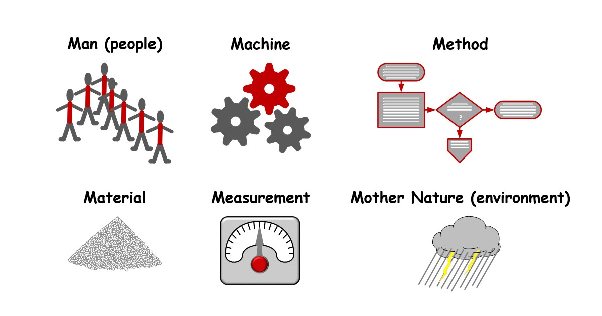
The 6-Ms from the Six Sigma discipline provide a context here for what potentially would influence variation in an LPBF process and therefore require quantification and control of their associated effects. 

  • Man (people): variation from how people do or observe things differently can affect a LPBF process, this is especially true for operator-intensive operations such as AM machine build-chamber cleanout, AM machine maintenance/calibration, material handling, and post-processing (to name just a few).
  • Machine: variation within the AM machine or between machines has direct effect on the LPBF process, which can be quantified as machine capability.
  • Method: variation in the design of the parts themselves, the LPBF process methods used during part fabrication, as well as post-processing and validation methods, have significant influence upon the quality of additively manufactured parts.
  • Material: raw material differences can have a major impact upon the LPBF process; different material types (e.g. titanium vs. stainless steel) require completely different process optimizations, and variation within material types (e.g. batch-to-batch from the same supplier or differences between batches from different suppliers) can influence the optimization enough to degrade the quality of the output parts.
  • Measurement: variation in the measurements made throughout the process, and especially at the process output, contribute to process uncertainty.
  • Mother Nature: environmental effects can influence the quality of the LBPF process output, for example, ambient humidity level has a large impact on the physical characteristics of the raw powder material.

Mitigating Risk From Process Variation

To address these concerns about variation in the process, Moog uses the PFMEA (Process Failure Modes Effects Analysis), which is based on theoretical knowledge from our M&PE (Materials and Process Engineering) experts, as well as the experiential knowledge gained over many years of AM development that resides within our AMC.  The PFMEA allows the risk for producing unacceptable parts to be quantified and mitigated though a set of actions that must be implemented for the identified risk factors. Often, structured studies (i.e. experimentation) are required to address the PFMEA risk mitigation, the scope of which is governed by the level of profound knowledge[1] that exists for the process in question. 

[1] See Dr. Deming’s Theory of Profound Knowledge

The Challenge of Studying Complex Processes

Variation arising from factors within each of the 6-M categories can interact with each other and also with factors from different categories.  As an example: humidity may have a greater effect upon one material type than another, which would represent an interaction between environmental and material factors.  Furthermore, these factors can either be crossed with or nested within other factors. For instance, several technicians may be involved with making measurements of samples of a process output, but if each technician only takes measurements within their own group of samples, the measurement-sample factor would be nested within the measurement-person factor.  Nested factors will not produce an interaction effect.

As shown in the tables below, when more and more LPBF factors are considered for study, the number of process output treatment combinations in the experimental space grows exponentially.  

Factors Levels Treatments Growth
1 2 2  
2 2 4 200%
3 2 8 400%
4 2 16 800%
5 2 32 1600%
6 2 64 3200%
7 2 128 6400%
8 2 256 12800%
Factors Levels Treatments Growth
1 3 3  
2 3 9 300%
3 3 27 900%
4 3 81 2700%
5 3 243 8100%
6 3 729 24300%
7 3 2187 72900%
8 3 6561 218700%
  • Studying four factors at two different levels for each factor (e.g. low and high) will produce 16 unique experimental treatment combinations, and doubling the factors to eight will increase the number of treatments to 256
  • Studying four factors at three different levels (e.g. low, nominal and high) will produce 81 unique experimental treatment combinations, and doubling the factors to eight will increase the number of treatments to 6561

Applied Industrial Statistics to the Rescue

At first, the rapid growth of the experimental space from the inclusion of additional factors appears overwhelming. Fortunately, there are several techniques from applied industrial statistics that can be used to address the problem of extracting unbiased information from complex systems.  Statistical Design of Experiments (DOE) provides a quantitative highly efficient approach to characterize and then optimize a multitude of process parameters.  Unlike one-factor-at-a-time (aka OFAT or 1FAT) testing, a DOE varies multiple factors simultaneously, and because each factor column in the experimental matrix is orthogonal with respect to the others, the factor main effects, as well as the factor interaction effects can be estimated independently (see the sidebar for additional information).

There are many different matrix designs used with DOE and normally, the nature of the experimental space such as the factor number, orthogonality, type and levels—as well as the response variables to be studied, will define the design of the experimental matrix and what error-control strategies are used.  The process development phase (e.g. parameter design studies or optimization for production) will also influence the experimental design.

DOE AM Sample Blocks for Within-Build-Plate Spatial Treatment Combinations

To determine which DOE factor effects are significant and therefore worthy of continuing study, and assuming adequate statistical degrees-of-freedom (DoF) have been allocated for the experimental error terms, the Analysis of Variation (ANOVA) is used to mathematically decompose the hypothetical sources of variation (e.g. factor main effects and factor interactions) from the output data vector (the response variable), and to quantify the level of experimental error (i.e. residual variation). The statistical F-test is used then used to determine if an observed effect has significance[2].


[2] Inadequate DoF will not preclude finding the significant experimental effects; as an example, the half-normal probability plot provides an excellent method for determining the significance of factors if ANOVA cannot be used (note that relying solely on the variation from unassigned columns in an experimental matrix as a substitute for error terms, can provide misleading information about the significance of factors in the ANOVA output).

Orthogonality and Design of Experiments

Two vectors are orthogonal if the sum of the products of their corresponding elements is 0 (i.e. the dot product of two vectors at 90° to each other). As an example, consider the vectors a & b:

a = [-4, 4, -4, 4]     b = [-10, -10, 10, 10]  

ab = -4(-10) + 4(-10) + -4(10) + 4(10)

ab = 40 - 40 - 40 + 40 = 0

In a DOE matrix, all column vectors are usually orthogonal, which results in the linear independence of the input variables, allowing unbiased responses from each main effect and interaction term to be estimated independently, despite simultaneous factor changes.

·       Full Factorial: all possible information can be obtained from a design (all main effects and higher order interactions)

·       Fractional Factorial: a subset of the information can be obtained from the design (typically all main effects and often, a subset of the interactions…depending on the fractionalization order)

A DOE matrix may also be balanced, which means the data are distributed uniformly over the design space by equalizing the number of levels for each factor.

·       The full factorial design is both orthogonal and balanced; however, balance is not a prerequisite attribute for a DOE matrix

·       DOE matrices such as the Central Composite Design (CCD), sacrifice balance in favor of a more optimized distribution of the predicted error

·       There are other classes of DOE that sacrifice both orthogonality and balance to enhance certain aspects of the information matrix, or to satisfy different constraints 

Cube Representation of a Three-Factor CCD Face-Centered DOE Matrix

Further Discussions

There are additional topics and challenges presented in the development and optimization of an LPBF process:

·         Some common DOE-based approaches


Click to read Issue #2 of this blog series > Issue #2: Process Development and Control in Metal Additive Manufacturing


Share this Article: