Issue 3.2 | Additive Manufacturing Machine and Measurement Capability Limitations
Click to read Issue #1 of this blog series > Issue #1: Process Development and Control in Metal Additive Manufacturing
Click to read Issue #2 of this blog series > Issue #2: Process Development and Control in Metal Additive Manufacturing
Click to read Issue #3.1 of this blog series > Issue #3.1: Process Development and Control in Metal Additive Manufacturing
This is a sidebar for Issue #3.1, which discusses the general effects of machine capability and measurement system accuracy (MSA) upon the additive manufacturing (AM) laser powder bed fusion (LPBF) process in Moog’s Additive Manufacturing Center (AMC). This article explores modeling techniques for the AM machine capability within a computer simulation of the LPBF specific energy density (Ed), using statistical Design of Experiments (DOE), and comparing this approach to the more traditional Monte Carlo and Sensitivity analysis methods.
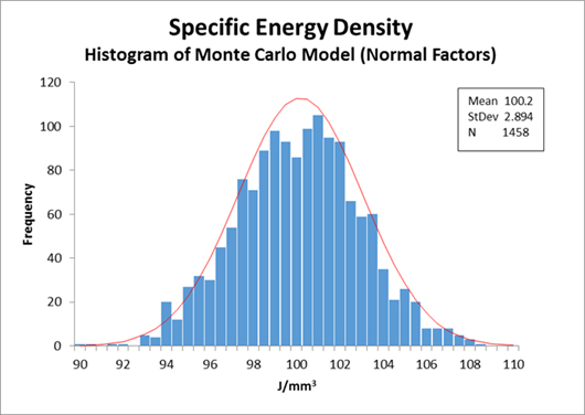
The histogram above represents effects from multiple sources of machine capability error upon the Ed of the LPBF AM process. At Moog, we have refined an equation-based coarse lumped-element model of Ed into a more detailed version that accounts for effects from the machine’s optics and other machine-specific settings; machine capability assessment (MCA) studies have been conducted in the AMC to quantify errors in the AM machine settings, and this information can be used in computer models to estimate the contribution of machine capability to process error. With normally-varied inputs based on MCA studies, the histogram shown above…as generated by a Monte Carlo Simulation (MCS)…indicates that the Ed can vary from the targeted setting by approximately ±9%.
The refined Ed model may also be studied through DOE to complement MCS, with the various process inputs exercised through an experimental matrix, and the model output Ed response analyzed through ANOVA (Analysis of Variation) and main effect and interaction plots instead of MCS output sensitivity analysis (SA). In this particular case, there are several advantages of using DOE for this model to understand the effects from uncertainties:
· The limitations imposed on DOE in the physical world (uncontrolled noise, limited samples due to costs, the need for replication and blocking) do not apply
· Using the Taguchi Robust Design ([1] Please see the links under ‘Additional Resources’ at the end of this article) approach, the components of variation can be studied simultaneously with process design parameters, with the uncertainty factors assigned to the outer-noise array.
· The output of a DOE-based computer simulation is often times more intuitive than MCS, which is important for the understanding of fellow stake holders and the decision makers in management
There are also several limitations to be aware of when using a DOE approach instead of the MCS:
· The variances produced in the model will be different for DOE and MCS unless a correction is used to correlate the two different outputs (see below)
· DOE levels do not work for one-sided distributions (typically associated with parameters that have no negative values)
The way to get around the first disadvantage is shown below, and for the one-sided parameters, the only solution possible is to include these parameters in the unassigned variation, and allow the factor setting to vary randomly following a Gamma or Weibull distribution.
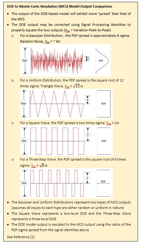
It is necessary to correct the output of a DOE to that of the MCS. This correction may be performed either at the inputs (DOE factor level settings) or at the outputs (DOE response) using identities that I have taken from electronic signal processing (see the sidebar).
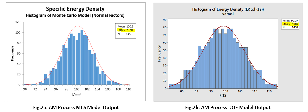
The histograms above show the MCS Ed model output on the left (Fig. 2a) DOE Ed model output the right (Fig. 2b). Notice that the model’s DOE output (run in a 3-level full factorial matrix) has a standard deviation (highlighted) of 7.086 J/mm3, which is about 245% greater than that of the model’s MCS output (with all parameters varied normally) with a standard deviation of 2.894 J/mm3 (highlighted). Using the signal-processing identities in the sidebar, we can show that this difference in variation between the two model outputs can be equated.
- The peak-to-peak variation (Vpp) of a three step wave = √6σDOE-3-Level
- And the Vpp of normal distribution = 6σMCS normal
Relating these two distributions 1-to-1:
- Vpp of a three step wave / Vpp of normal distribution = 1
- √6σDOE 3 Level / 6σMCS normal = 1 and σDOE 3 Level = ( 6 / √6 ) x σMCS normal ∴ σDOE 3 Level ≈ 2.45 x σMCS normal
Checking the two distributions from the model outputs:
- σDOE 3 Level = 7.086 and σMCS normal = 2.894 ∴ σDOE 3 Level / σMCS normal = 7.086 / 2.894 = 2.449 ≈ 2.45
(multiple runs will vary this ratio around 2.45 within the standard error of the estimate)
Therefore, in the example above, the output of the 3-level DOE model is approximately 245% wider than a MCS using the same factors varied with random normally-distributed input, and to translate the DOE output variation to equivalent MCS output, the DOE must be rescaled by 1/2.45 (40.8%). For this example, the adjustment could also be made by reducing each of the input factor level separations to 41% of the expected spread from the lack-of-capability of each factor setting. This approach will allow the variation in a system to be modeled using DOE, which will output much more information than a MCS, but still allow the output spread of the DOE-based model to be related to the equivalent MCS output without the need to run a separate MCS. I have found that this comparison is necessary in order to answer the inevitable questions that come up about what the MCS output would look like. Again, the DOE approach works for this specific Ed model, and the limitations discussed previously need to be accommodated.